Advent of Code 2019 in 130 ms: day 19
Day 19: Tractor Beam
Day 19 is another Intcode challenge, and in terms of performance optimization it is much like day 15 in that the focus is on minimizing the number of calls to the Intcode program. My solution uses linear approximation followed by binary search, and runs in 1.3 ms.
Part 1 establishes the basic tools we need: a naïve solution could simply iterate through the whole space and check each point, but we can work much faster by only exploring the edges of the beam. Once we know the width of the beam at each y coordinate, we can easily compute its volume.
  0   x ->
0 #.............................
  ..............................
y ..............................
  ..#...........................
| ...#..........................
v ....#.........................
  ....##........................
  .....#........................
  ......#.......................
  ......##......................
  .......##.....................
  ........##....................
  ........###...................
  .........##...................
  ..........##..................
  ..........###.................
  ...........###................
  ............###...............
  ............####..............
  .............###..............
  ..............###.............
  ..............####............
  ...............####...........
  ................####..........
  ................#####.........
  .................####.........
  ..................####........
  ..................#####.......
  ...................#####......
  ....................#####.....
As we can see in figure 12, the beam is roughly cone-shaped,
which I assume to be true for any puzzle input.
At the very beginning there’s a sneaky gap in the beam
which we’ll have to account for,
but we can devise a simple algorithm for following the edges.
To find the right edge of the beam going downward (increasing y),
start at the x coordinate of the edge at the previous row,
and walk to the right while the current coordinate is within the beam.
To find the left edge, similarly start at the previous coordinate
and walk right until the current coordinate is within the beam.
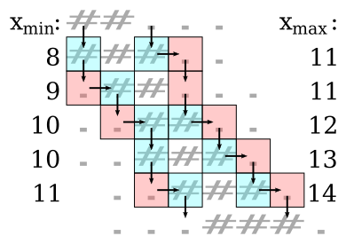
This algorithm is illustrated in figure 13;
note that x_min is the first coordinate inside the beam
and x_max is the first coordinate outside the beam.
This makes it easy to compute the beam width.
There’s one edge case where this fails: that sneaky gap at the beginning.
Because of that, if our max-edge algorithm starts on a non-beam coordinate
it will instead walk left until it finds a beam coordinate.
The min-edge algorithm can be simpler:
if we don’t find the beam within, say, 10 steps of the starting coordinate,
just give up and return zero.
With that, for part 1 we just need to find the x_min and x_max
for each y = 0, 1, ..., 49, and compute the sum of x_max - x_min for each row.
Part 2 gets a little more interesting.
Now we need to find the point (x0, y0) closest to the origin
such that the square between (x0, y0) and (x0 + 100, y0 + 100) fits into the beam.
With a bit of geometric imagination, shown in figure 14,
we can find that any such square must and will satisfy the condition
that both (x0 + L - 1, y0) and (x0, y0 + L - 1) are within the beam,
where L = 100 is the desired width of the square.

This means that given a point on the right edge of the beam,
we only need to check a single other point to know whether a square
with its top-right corner at the first point will fit in the beam.
The problem now becomes finding the smallest y0 for which (x_max - 1, y0)
is such a point.
We can do this with a simple linear search; this took ~14 ms for my program to compute.
But if we model the beam as roughly cone-shaped, we can make an initial guess
to skip ahead to a region where the solution is more likely to be.
Part 1 already has us compute x_min and x_max for the first 50 rows.
We can use these values to estimate the slope of the beam edges:
k1 = x_max / 49 for the right edge and k2 = x_min / 49 for the left edge.
This gives us two linear functions:
x_min(y) = y * k2 and x_max(y) = y * k1.
If we combine these with the square criterion, we get
x_max(y0) - x_min(y0 + L - 1)    >= L
y0 * k1 - (y0 + L - 1) * k2      >= L
y0 * k1 - y0 * k2 - (L - 1) * k2 >= L
y0 * (k1 - k2)                   >= L + (L - 1) * k2
y0 * (k1 - k2)                   >= L + L * k2 - k2
y0 * (k1 - k2)                   >= L * (1 + k2) - k2

y0 >= (L * (1 + k2) - k2) / (k1 - k2)
This gives us a fairly good first approximation of y0, which we can now refine.
We can just linear search from this guess forward or backward,
depending on whether our square fits at the guessed y0;
this takes my program about 2.5 ms.
Even faster, though, is a binary search.
We can start with 50 and our guess times 2 as the lower and upper limits.
We check the middle point and set either the upper or the lower limit
equal to the middle point, depending on if our guess was too high or too low.
We repeat this until the upper and lower limits meet,
which takes log2(max - min) steps.
This brings us down to 1.3 ms total for both parts.